View Source

Overview

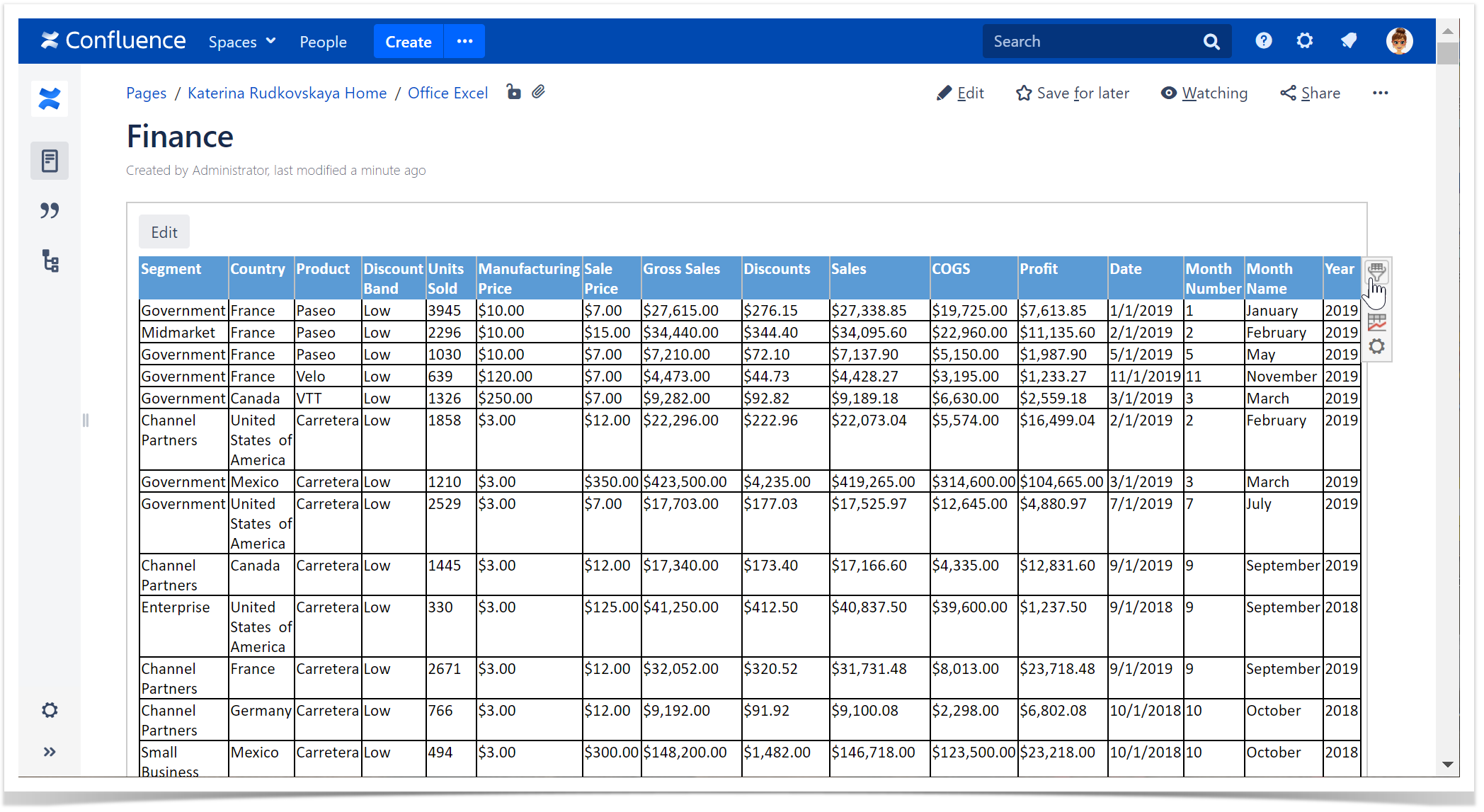
The Source Table:

Table Filter, Charts & Spreadsheets for Confluence > How to use the app with Office Excel > image2020-2-19_13-24-12.png

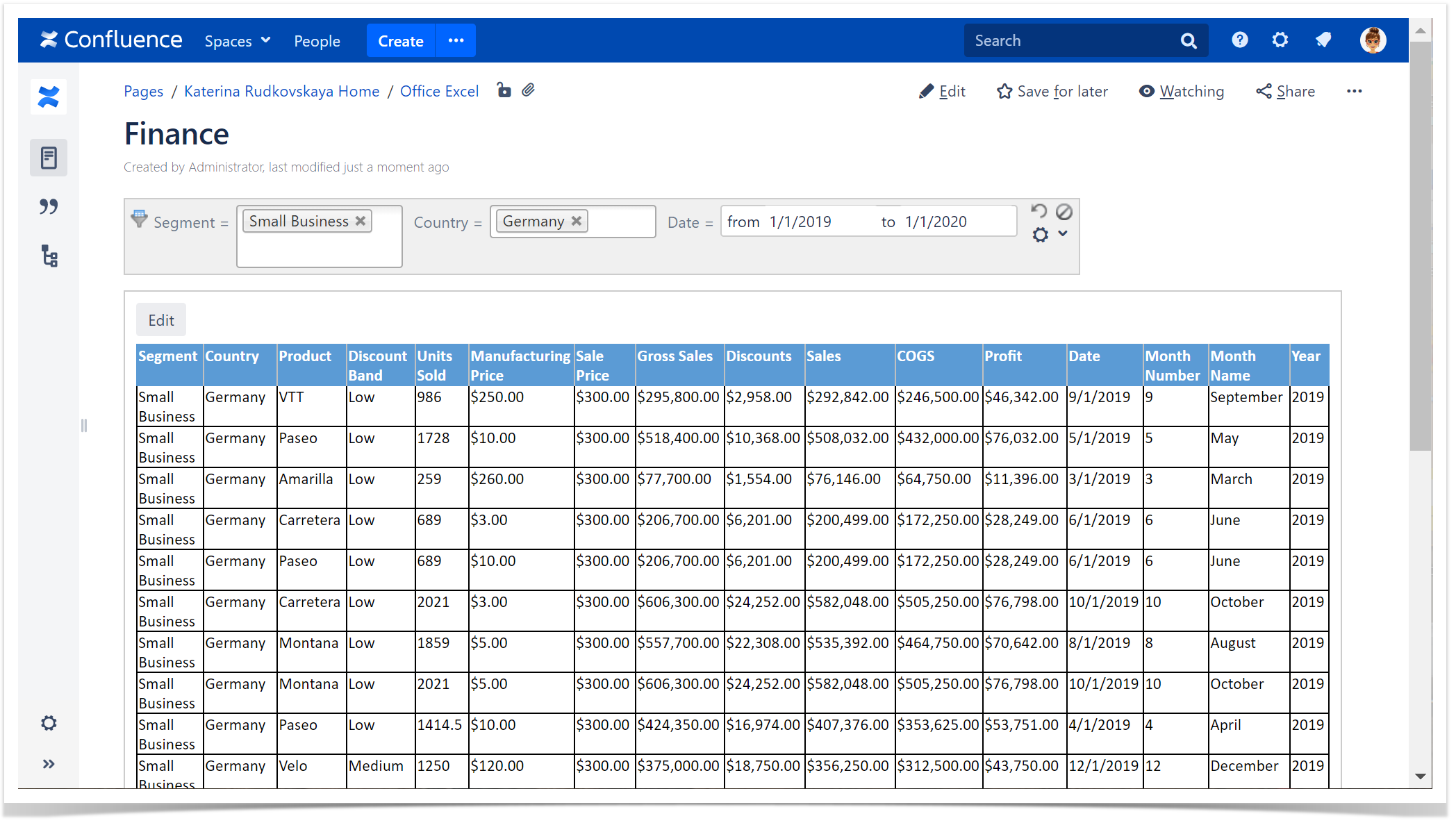
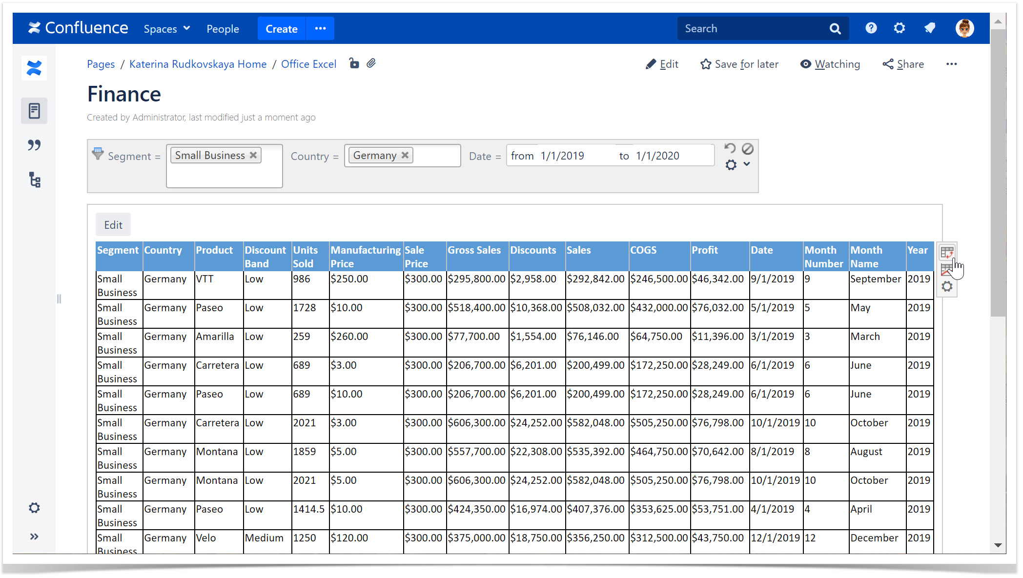
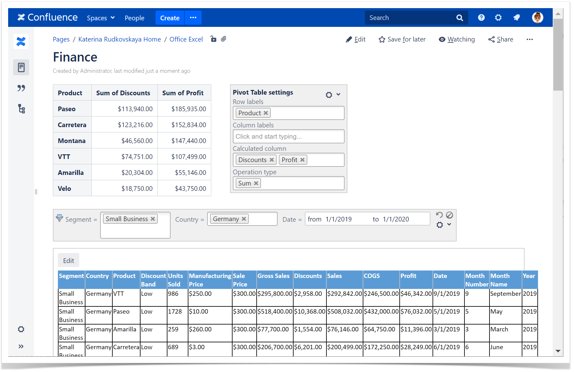
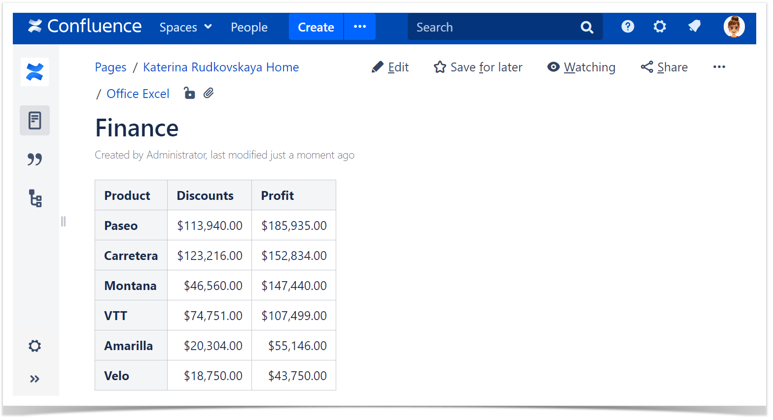
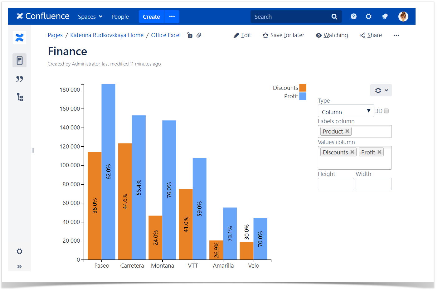
The Result:

Table Filter, Charts & Spreadsheets for Confluence > How to use the app with Office Excel > image2020-2-19_14-31-5.png

Create the Office Excel macro to display the content of an Excel spreadsheet on a page and configure its parameters.

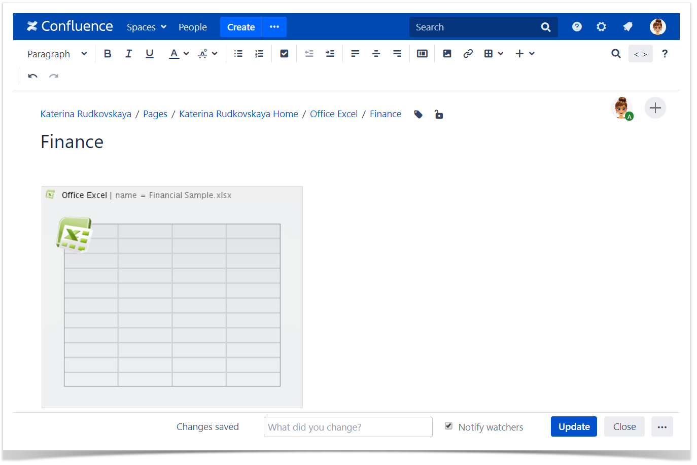
Table Filter, Charts & Spreadsheets for Confluence > How to use the app with Office Excel > 3.png

Table Filter & Office Excel

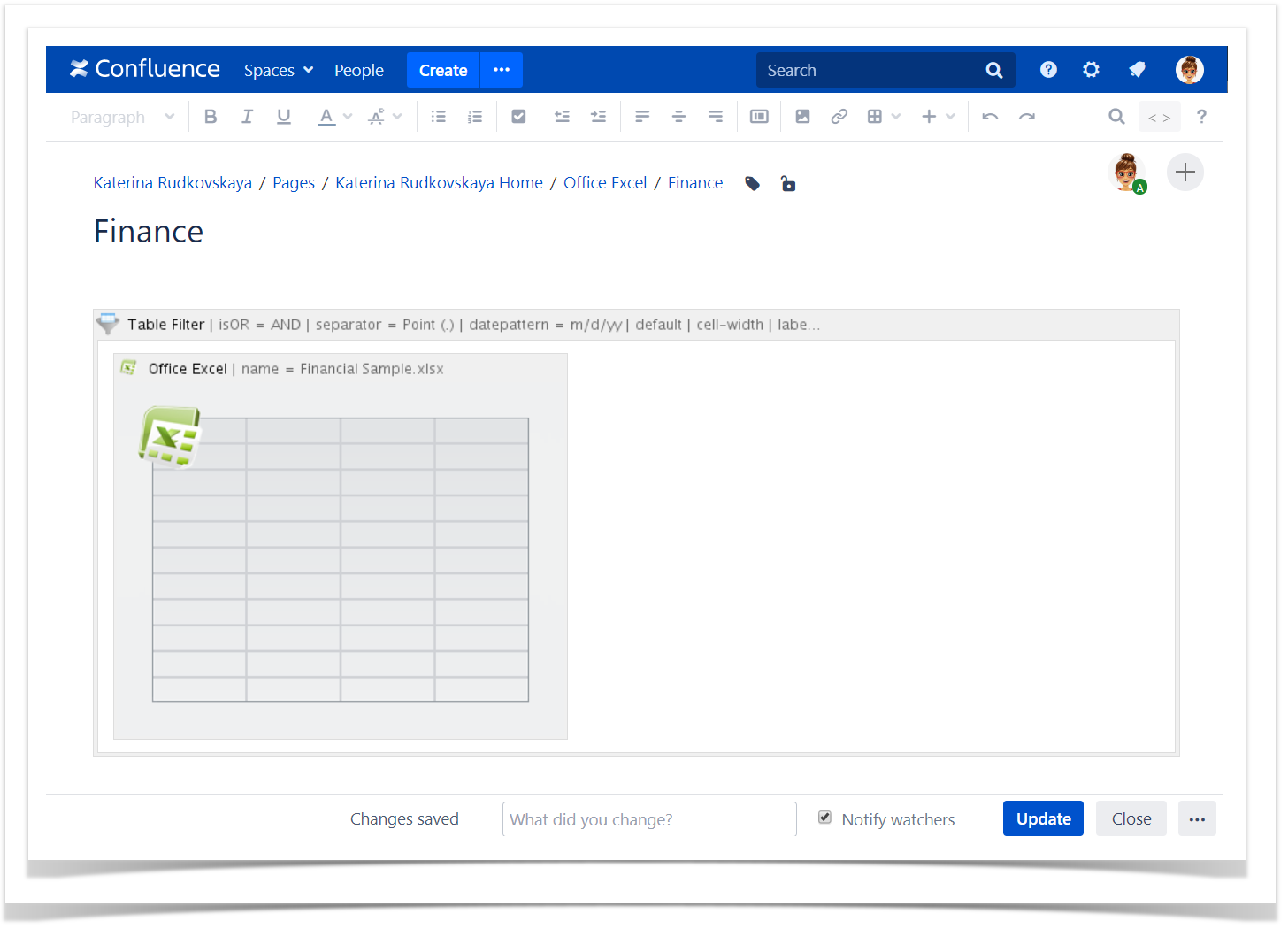
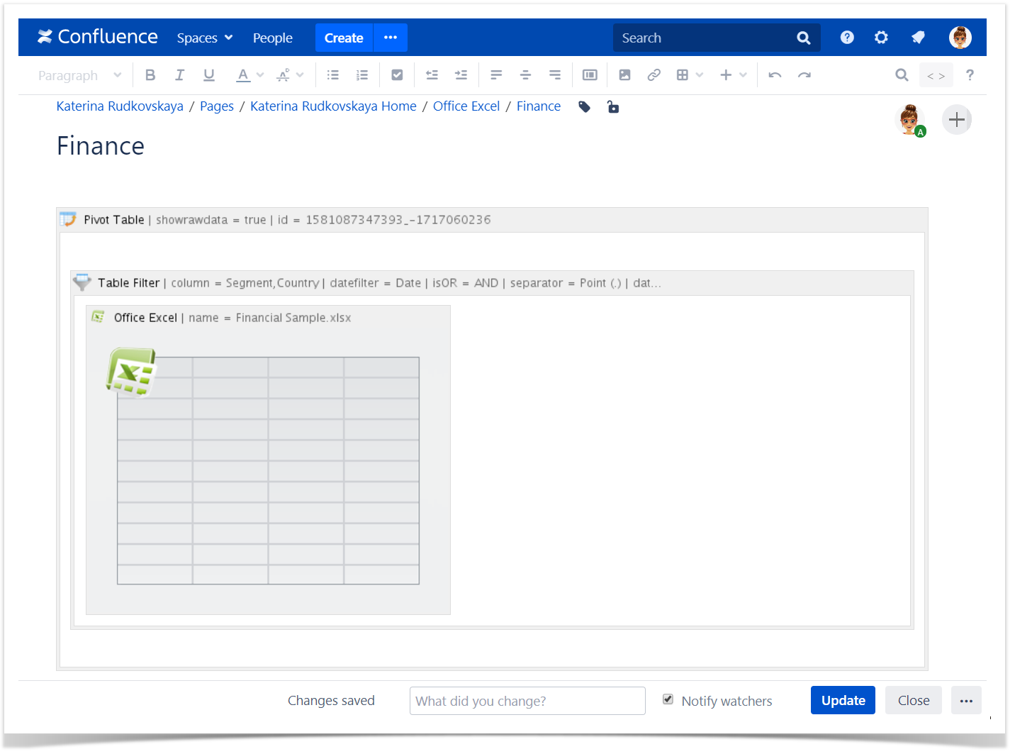
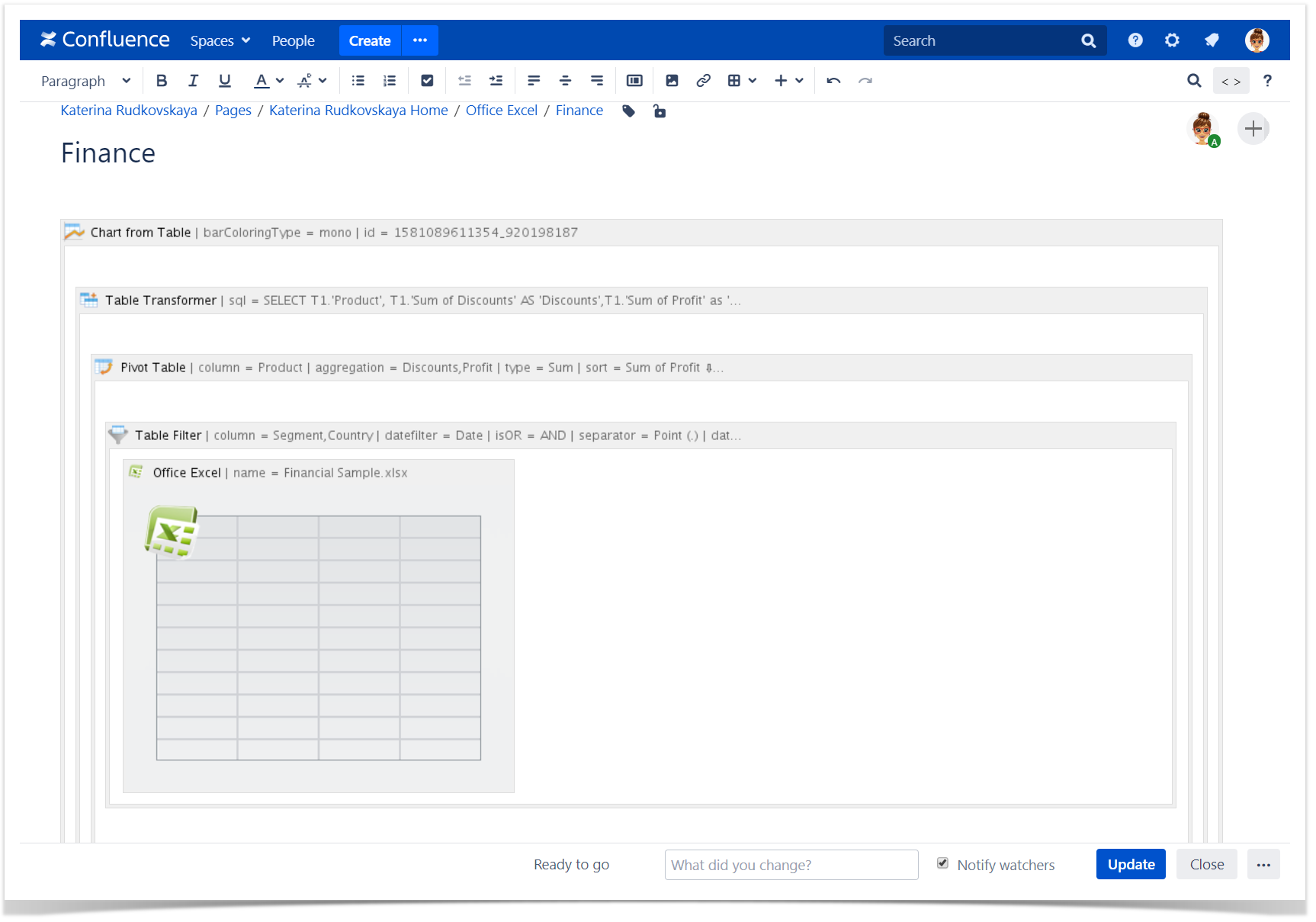
1. Add the Table Filter macro to the Office Excel macro.

Table Filter helps you to filter data, set default sorting , freeze rows and columns , calculate totals and more.

2. Add filters to the table columns and set filter values.

Default sorting in the Table Filter macro can't be applied as Sorting in the header row doesn't work with tables outputted by the Office Excel macro in Confluence by default.

Table Filter, Charts & Spreadsheets for Confluence > How to use the app with Office Excel > 4.1.png

Table Filter, Charts & Spreadsheets for Confluence > How to use the app with Office Excel > 4.png

Table Filter, Charts & Spreadsheets for Confluence > How to use the app with Office Excel > 4.2.png

Pivot Table & Office Excel

3. Add the Pivot Table to the Office Excel macro with filtered data.

Pivot Table allows you to summarize and aggregate your table data.
You can select the following operations: Sum, Count, Min, Max, Average, Literal.

4. Configure the pivot table.

Table Filter, Charts & Spreadsheets for Confluence > How to use the app with Office Excel > 5.png

Table Filter, Charts & Spreadsheets for Confluence > How to use the app with Office Excel > 5.1.png

Table Filter, Charts & Spreadsheets for Confluence > How to use the app with Office Excel > 5.2.png

Table Transformer & Office Excel

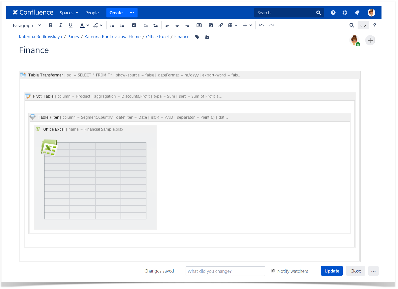
5. Add the Table Transformer macro to the filtered and aggregated Excel table.

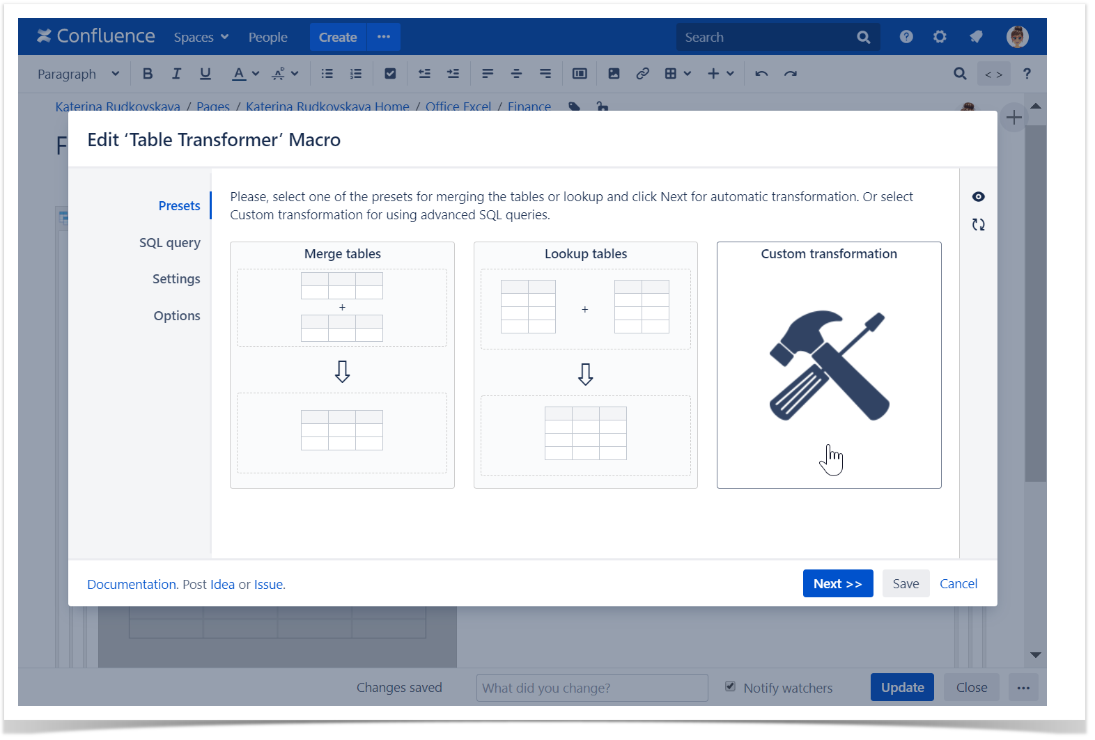
You can place one or multiple tables within the macro body to merge, look up them or to perform custom calculations.

6. Select one of the presets or switch to the SQL query tab.

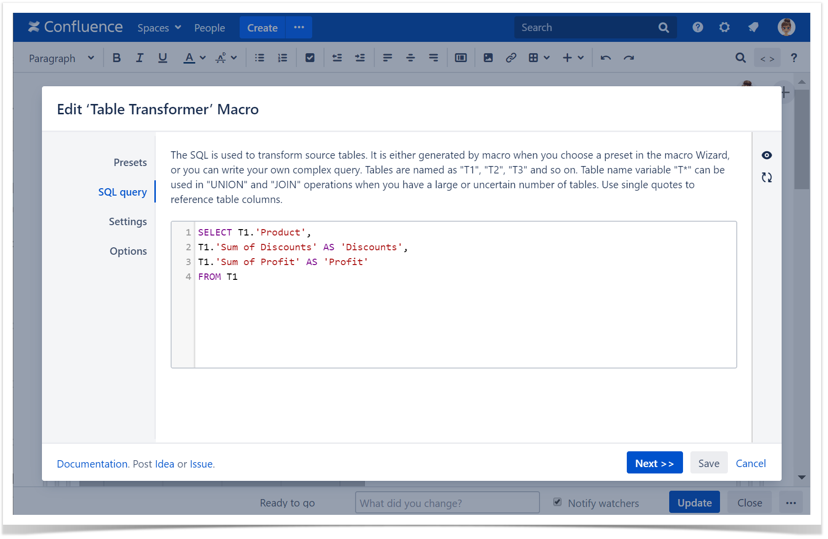
Table Filter, Charts & Spreadsheets for Confluence > How to use the app with Office Excel > 6.png

Table Filter, Charts & Spreadsheets for Confluence > How to use the app with Office Excel > 6.1.png

7. Enter the following SQL query to rename columns in the pivot table:

SELECT T1.'Product',                                     
T1.'Sum of Discounts' AS 'Discounts', 
T1.'Sum of Profit' AS 'Profit'
FROM T1

Table Filter, Charts & Spreadsheets for Confluence > How to use the app with Office Excel > 7.png

Table Filter, Charts & Spreadsheets for Confluence > How to use the app with Office Excel > 7.1.png

Chart from Table & Office Excel

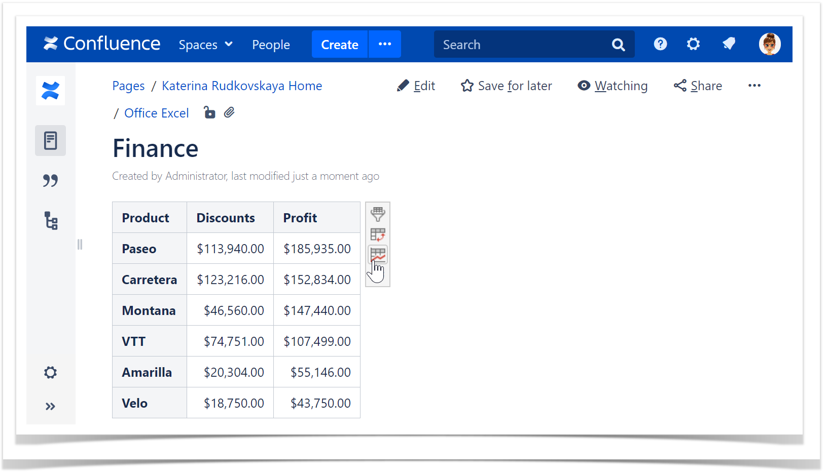
8. Add the Chart from Table macro to the already filtered, aggregated and transformed Excel table to visualize data with the help of charts and graphs.

9. Set the parameters of the chart .

Table Filter, Charts & Spreadsheets for Confluence > How to use the app with Office Excel > 8.png

Table Filter, Charts & Spreadsheets for Confluence > How to use the app with Office Excel > 8.1.png

Table Filter, Charts & Spreadsheets for Confluence > How to use the app with Office Excel > 8.2.png

You can change the filtration criteria, the pivot table and chart parameters on the fly.
The changes will be automatically applied to the data from the Office Excel macro.

The Office Excel macro can be used with each of the macros separately or combined with them according to your needs.